Data Analysis Notebook - How to bring in data from a Gen3 Data Commons to the workspace and perform data analysis

1. Introduction to the Open Access Data Commons

  • The Open Access Data Commons https://gen3.datacommons.io/ supports the management, analysis and sharing of data for the research community with the aim of accelerating discovery and development of diagnostics, treatment and prevention of diseases.
  • Gen3 Data Commons store a) data files and b) structured metadata.
  • For the first part of this notebook (sections 2 and 3), we show how to download data files and bring them to the workspace using the Gen3-client and in the second part below (section 4), we will show how to download structured metadata to the workspace using the Gen3 Python SDK.

2. Download data files from the Gen3 Data Commons and bring them to the workspace

2.1 Introduction to the dataset

  • We will analyze two data files ('GSE63878_final_list_of_normalized_data.txt.gz' and 'pheno_63878_2.txt') from the study "GEO-GSE63878".
  • This study deals with peripheral blood leukocytes gene expressions which were subject to transcriptional analysis for 48 service members both prior-to and following deployment to conflict zones. Half of the subjects returned with Post-traumatic Stress Disorder (PTSD), while the other half did not.

2.2 Importing the data files to the workspace using the Gen3-client: a step-by-step guide

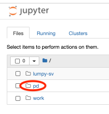
  • First, we can find and browse all data files stored on the Gen3 Data Commons under the "Files" tab on the Data Exploration page.
  • To download data files, we will create and download a file manifest, which is a light JSON file that is called by the Gen3-client to download all enlisted entities to the workspace:

  • In the Explorer under the "Files" tab we find the "Data Format" category; from here we can select the box next to "TXT" that builds a cohort and shows all files in the Data Commons that end on "TXT". In this case: 'GSE63878_final_list_of_normalized_data.txt.gz' and 'pheno_63878_2.txt'.

  • We click on "Download (File) Manifest", save it to our local drive, and upload it to the workspace under the /pd directory as "file-manifest.json". For help on this step, see the screen recordings shown here.
  • Only the files in the /pd directory will persist in the cloud after workspace termination.
  • We visit now the profile page, click on "Create API key", download the .JSON file and upload this "credentials.json" to the workspace under the /pd directory.
  • In the workspace, we open a new terminal.
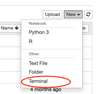
  • We run the following commands in the terminal (also shown here) to download and install the Gen3-client, configure the profile "demo" with the "credentials.json", and to download the data files calling the "file-manifest.json":
- wget https://github.com/uc-cdis/cdis-data-client/releases/download/2020.11/dataclient_linux.zip
- unzip dataclient_linux.zip
- PATH=$PATH:~/

- gen3-client configure --apiendpoint=https://gen3.datacommons.io --profile=demo --cred=~/pd/credentials.json
- cd pd
- gen3-client download-multiple --profile=demo --manifest=file-manifest.json --skip-completed
  • The two files should be now saved in the /pd directory. You can terminate the terminal session.

Note. If you want to download only a single data file the Gen3-client command changes as shown here. You can also find the data file on the Exploration Page and click on the file's GUID to "Download".

3. Load and analyze the data files here in the workspace

  • For this section, you need to start running a jupyter python notebook and run the code snippets below.

3.1 Install dependencies and import python libraries

In [1]:
# Uncomment the lines to install libraries if needed.
# !pip install numpy
# !pip install matplotlib
# !pip install pandas
# !pip install seaborn
In [1]:
# Import libraries:
import pandas as pd
import numpy as np
import matplotlib.pyplot as plt
import matplotlib as mpl
import os
import seaborn as sns
import re
from pandas import DataFrame
import warnings
warnings.filterwarnings("ignore")
import gzip
import scipy
import sys
import sklearn
import random
import math

3.2 Unzip data file

In [ ]:
!gzip -dk 'GSE63878_final_list_of_normalized_data.txt.gz' # command -k saves the original zipped file

3.3 Load the first txt file as a Pandas dataframe "pheno_df"

This dataframe shows the characteristics, sample descriptions, etc. associated with measured gene expression.

In [2]:
pheno_df = pd.read_csv('/home/jovyan/pd/pheno_63878_2.txt', sep='\t')
pheno_df.head() # show top 5 rows of dataframe
Out[2]:
Source Name Comment [Sample_description] Comment [Sample_source_name] Comment [Sample_title] Characteristics [cell type] Characteristics [condition] Term Source REF Term Accession Number Characteristics [individual] Characteristics [organism] ... Normalization Name Derived Array Data File Comment [Derived ArrayExpress FTP file] FactorValue [condition] Term Source REF.9 Term Accession Number.2 FactorValue [individual] FactorValue [time-point] Time PTSD
0 GSM1558870 1 Sample48_3 Human peripheral blood leukocytes, control, po... Control Post 48 peripheral blood leukocytes control EFO EFO_0001461 48 Homo sapiens ... GSM1558870_sample_table.txt norm GSM1558870_sample_table.txt ftp://ftp.ebi.ac.uk/pub/databases/microarray/d... control EFO EFO_0001461 48 post-deployment 2 1
1 GSM1558869 1 Sample48_1 Human peripheral blood leukocytes, control, pr... Control Pre 48 peripheral blood leukocytes control EFO EFO_0001461 48 Homo sapiens ... GSM1558869_sample_table.txt norm GSM1558869_sample_table.txt ftp://ftp.ebi.ac.uk/pub/databases/microarray/d... control EFO EFO_0001461 48 pre-deployment 1 1
2 GSM1558868 1 Sample47_3 Human peripheral blood leukocytes, control, po... Control Post 47 peripheral blood leukocytes control EFO EFO_0001461 47 Homo sapiens ... GSM1558868_sample_table.txt norm GSM1558868_sample_table.txt ftp://ftp.ebi.ac.uk/pub/databases/microarray/d... control EFO EFO_0001461 47 post-deployment 2 1
3 GSM1558867 1 Sample47_1 Human peripheral blood leukocytes, control, pr... Control Pre 47 peripheral blood leukocytes control EFO EFO_0001461 47 Homo sapiens ... GSM1558867_sample_table.txt norm GSM1558867_sample_table.txt ftp://ftp.ebi.ac.uk/pub/databases/microarray/d... control EFO EFO_0001461 47 pre-deployment 1 1
4 GSM1558866 1 Sample46_3 Human peripheral blood leukocytes, control, po... Control Post 46 peripheral blood leukocytes control EFO EFO_0001461 46 Homo sapiens ... GSM1558866_sample_table.txt norm GSM1558866_sample_table.txt ftp://ftp.ebi.ac.uk/pub/databases/microarray/d... control EFO EFO_0001461 46 post-deployment 2 1

5 rows × 45 columns

3.4 Load the second txt file as a Pandas dataframe "rna_df"

This dataframe shows genome expressions. Numbers after "Sample_" indicate pre-deployment ("1") and post-deployment ("3").

In [3]:
os.chdir('/home/jovyan/pd')
rna_df = pd.read_csv('/home/jovyan/pd/GSE63878_final_list_of_normalized_data.txt', sep='\t')
rna_df.head()
Out[3]:
Probe ID Gene Symbol Sample1_1 Sample1_3 Sample2_1 Sample2_3 Sample3_1 Sample3_3 Sample4_1 Sample4_3 ... Sample46_3 Sample47_1 Sample47_3 Sample48_1 Sample48_3 Unnamed: 98 Unnamed: 99 Unnamed: 100 Unnamed: 101 Unnamed: 102
0 8066716 ELMO2 9.137931 7.879140 8.706623 8.413021 8.871833 7.684935 9.283664 8.278483 ... 8.542750 8.799327 8.998155 8.677686 8.756859 NaN NaN NaN NaN NaN
1 8030368 RPS11 11.924280 11.573510 11.799527 11.755598 12.007807 11.758845 11.930047 11.928939 ... 12.123981 11.995779 12.017707 12.050722 12.107991 NaN NaN NaN NaN NaN
2 7980044 PNMA1 7.015597 6.370872 6.821562 6.638079 6.968514 6.326143 6.848688 6.813374 ... 6.868656 6.924999 6.867908 6.782773 7.067915 NaN NaN NaN NaN NaN
3 7940479 TMEM216 7.503816 5.972232 7.194987 6.272724 7.196858 6.401971 7.143758 6.802013 ... 6.614511 6.913884 7.471228 6.982341 7.057705 NaN NaN NaN NaN NaN
4 8066279 ZHX3 6.344508 6.955141 6.720097 6.787643 6.648538 6.777332 6.500822 6.544580 ... 6.824411 6.714426 6.355158 6.598794 6.505404 NaN NaN NaN NaN NaN

5 rows × 103 columns

3.5 Prepare the second dataframe rna_df (e.g. data cleaning)

In [4]:
rna_df = rna_df.dropna(1) # remove columns that contain "NaN"
del rna_df['Probe ID'] # delete first column for further analysis.
all_genes = set(rna_df["Gene Symbol"].to_list()) # save this column as list for further analysis.

3.6 Organize pheno_df and rna_df data into categories and combine

In [5]:
# list(pheno_df.columns) 
trim_pheno_df = pheno_df[['Comment [Sample_description]', 'Characteristics [condition]', 'FactorValue [time-point]']] # select columns to be worked with
trim_pheno_df.head()
Out[5]:
Comment [Sample_description] Characteristics [condition] FactorValue [time-point]
0 Sample48_3 control post-deployment
1 Sample48_1 control pre-deployment
2 Sample47_3 control post-deployment
3 Sample47_1 control pre-deployment
4 Sample46_3 control post-deployment
In [6]:
# Add the categories to the dataset 
blank = [name for name in rna_df.columns] # list all headers in rna_df

# Category "condition"
condition = (trim_pheno_df['Characteristics [condition]']).tolist() # move all rows of this column into a list
condition = condition[::-1] # switch as column Characteristics [condition] begins with sample48_3 instead of Sample1_1
condition.insert(0, 'condition') # add header 
ptsd = {col:val for col, val in zip(blank, condition)} # match headers from rna_df to 'condition'

# Category "deployment"
deployment = (trim_pheno_df['FactorValue [time-point]']).tolist()
deployment = deployment[::-1]
deployment.insert(0, 'deployment')
deploy = {col:val for col, val in zip(blank, deployment)}

Attention: **The next two code snippets should be run only once.**

In [7]:
# Adding category lists to the rna_df dataframe
# This will combine both datasets
rna_df = rna_df.append(ptsd, ignore_index=True)  # run only once
rna_df = rna_df.append(deploy, ignore_index=True) # run only once
rna_df.tail() # shows the last 5 rows of the dataframe
Out[7]:
Gene Symbol Sample1_1 Sample1_3 Sample2_1 Sample2_3 Sample3_1 Sample3_3 Sample4_1 Sample4_3 Sample5_1 ... Sample44_1 Sample44_3 Sample45_1 Sample45_3 Sample46_1 Sample46_3 Sample47_1 Sample47_3 Sample48_1 Sample48_3
10181 SLC39A6 8.24209 7.17973 7.79949 7.60747 7.92649 7.31457 7.8781 7.71006 8.41737 ... 8.26862 7.45759 7.47875 8.39298 7.92523 7.82593 8.13023 8.41975 8.00268 7.96456
10182 SNRPD2 8.1895 7.62186 7.92915 7.70063 8.2255 7.59012 7.76954 7.70023 8.05942 ... 8.43709 7.79318 7.95529 7.9854 7.95592 8.17159 7.93 7.92019 8.01057 8.13519
10183 CTSC 10.444 9.77531 10.2586 9.72933 10.3202 9.74488 10.7405 10.1667 10.4375 ... 10.4621 9.83597 10.0497 10.5271 10.1621 10.1144 10.5917 10.7041 10.3741 10.3844
10184 condition case (PTSD risk) case (PTSD) case (PTSD risk) case (PTSD) case (PTSD risk) case (PTSD) case (PTSD risk) case (PTSD) case (PTSD risk) ... control control control control control control control control control control
10185 deployment pre-deployment post-deployment pre-deployment post-deployment pre-deployment post-deployment pre-deployment post-deployment pre-deployment ... pre-deployment post-deployment pre-deployment post-deployment pre-deployment post-deployment pre-deployment post-deployment pre-deployment post-deployment

5 rows × 97 columns

In [8]:
# Transpose and relabel for easy wrangling
trans = rna_df.transpose()
trans.columns = trans.iloc[0] # [0] is the gene symbol row
trans = trans.drop(trans.index[0]) # only run once, or you'll start losing genes 
trans.head()
Out[8]:
Gene Symbol ELMO2 RPS11 PNMA1 TMEM216 ZHX3 ERCC5 PDCL3 DECR1 CADM4 RPS18 ... SELO GOLGA8B RAB8A PCIF1 PIK3IP1 SLC39A6 SNRPD2 CTSC condition deployment
Sample1_1 9.13793 11.9243 7.0156 7.50382 6.34451 8.50401 6.51273 9.07524 7.17572 10.4082 ... 8.59976 7.81222 9.43908 9.0422 8.63562 8.24209 8.1895 10.444 case (PTSD risk) pre-deployment
Sample1_3 7.87914 11.5735 6.37087 5.97223 6.95514 7.90332 5.62645 8.55404 6.94569 10.2794 ... 7.92597 7.71653 8.00783 8.11592 8.13457 7.17973 7.62186 9.77531 case (PTSD) post-deployment
Sample2_1 8.70662 11.7995 6.82156 7.19499 6.7201 8.42773 6.30857 9.02177 7.07879 10.5628 ... 8.29128 8.00509 9.53683 8.6407 8.58806 7.79949 7.92915 10.2586 case (PTSD risk) pre-deployment
Sample2_3 8.41302 11.7556 6.63808 6.27272 6.78764 8.28691 5.56848 8.66914 7.00094 10.6323 ... 8.2166 8.31954 8.41639 8.21003 8.3962 7.60747 7.70063 9.72933 case (PTSD) post-deployment
Sample3_1 8.87183 12.0078 6.96851 7.19686 6.64854 8.67884 6.50687 8.82516 6.95107 10.7497 ... 8.58784 8.05394 9.08206 8.85754 8.89265 7.92649 8.2255 10.3202 case (PTSD risk) pre-deployment

5 rows × 10186 columns

3.7 Statistical analysis on data

  • First we define the analysis functions and then we plot the data.

3.7.1 Processing dataframe

In [9]:
# Import libraries
import scipy
import sys
import sklearn
import random
import math

# Define function
def process_data(expression_df, condition, control, experimental):
    #expresion_df = input is the dataframe that we have defined above, gene expressions before and after deployment
    #condition = choose condition; for example separate your dataframe between between condition and deployment; input as string
    #control = control variable; input as string
    #experimental = experimental variable, input as string
    #returns dataframe of gene names, mean values, log2fold change, p-value, -log10(pval), and all replicates for each gene

    experimental_df = expression_df[expression_df[condition].str.contains(experimental)]
    experimental_df = expression_df.drop(columns=['condition', 'deployment'])
    control_df = expression_df[expression_df[condition].str.contains(control)]
    control_df = control_df.drop(columns=['condition', 'deployment'])

    deg_genes = {} # dictionary of final data
    gene_names = list(experimental_df.columns)
    for gene in gene_names:
        ex_mean = experimental_df[gene].mean() # experimental mean
        ctrl_mean = control_df[gene].mean() # control mean
        ex_reps = experimental_df[gene] # all replicates of PTSD samples
        control_reps = control_df[gene] # all replicates of control samples
        pval = scipy.stats.ttest_ind(control_reps, ex_reps) # calculate pval
        pvalue = pval.pvalue # gets specific p-value, removes meta data
        gene_data = {
            'GeneNames': gene,
            'ctrl_mean': ctrl_mean,
            'ex_mean': ex_mean,
            'log2(foldchange)': math.log2(ex_mean) - math.log2(ctrl_mean),
            'p-value': pvalue, #gets only the p-val
            '-log10(p-value)': math.log10(pvalue) * (-1),
            'ctrl_reps': control_reps.values.tolist(),
            'experimental_reps': ex_reps.values.tolist()
        }

        deg_genes[gene] = gene_data

    deg_data_frame = pd.DataFrame.from_dict(deg_genes, orient='index')

    return(deg_data_frame)
In [10]:
# Returns dataframe of gene names, means, log2fold change, p-value, -log10(pval), and all replicates for each gene
deg_data_frame = process_data(trans, 'condition', 'control', 'PTSD')
deg_data_frame.reset_index(drop=True)
Out[10]:
GeneNames ctrl_mean ex_mean log2(foldchange) p-value -log10(p-value) ctrl_reps experimental_reps
0 1-Mar 9.510892 9.532068 0.003208 0.687208 0.162912 [9.410044466, 9.107843367000001, 9.366556499, ... [9.609778596, 9.105890847000001, 9.562257875, ...
1 1-Sep 9.076845 9.053272 -0.003752 0.676129 0.169970 [9.032684824, 8.335088326000001, 9.058631866, ... [9.16795825, 7.8387380229999994, 9.01605535299...
2 10-Sep 5.999581 5.977097 -0.005417 0.645976 0.189784 [5.868845003, 6.151832213, 5.237751485, 5.6133... [5.893990292000001, 5.981416566, 5.474670931, ...
3 11-Sep 8.466428 8.468044 0.000275 0.973021 0.011878 [8.480006652, 7.933843997, 8.143054023, 7.9811... [8.509015495, 7.844778159, 8.445299485, 8.3667...
4 14-Sep 9.287598 9.281226 -0.000990 0.912520 0.039758 [9.137119174, 8.947042253, 9.440136676, 9.0133... [9.067632567999999, 9.070145062, 8.910505062, ...
5 15-Sep 10.469146 10.464646 -0.000620 0.874873 0.058055 [10.28441173, 10.17050459, 10.17577238, 10.345... [10.33314355, 10.12164928, 10.33216856, 10.225...
6 2-Mar 8.610877 8.610415 -0.000077 0.994711 0.002303 [8.698068812999999, 7.894693602, 7.98176665, 8... [8.910645377, 8.031103538, 8.216321252, 8.0965...
7 2-Sep 9.527714 9.506905 -0.003154 0.680029 0.167473 [9.52285479, 8.917381702, 9.111436143999999, 8... [9.661669016, 8.838995168, 9.336902379, 9.1733...
8 3-Mar 7.889784 7.892823 0.000556 0.954027 0.020439 [7.987255996, 7.407566161, 7.820764324, 7.5369... [7.829274094, 7.129441302, 7.474798702999999, ...
9 5-Mar 7.849298 7.874746 0.004670 0.532610 0.273591 [8.017721647, 7.531838991, 7.684344511, 7.5517... [8.198870231, 7.3032367979999995, 7.806763694,...
10 6-Mar 10.031418 10.011277 -0.002900 0.538935 0.268463 [10.03900751, 9.881189016, 9.829074808, 9.2741... [10.08295039, 9.712522479, 9.990016302999999, ...
11 6-Sep 9.543408 9.555600 0.001842 0.832689 0.079517 [9.361915924, 8.980524698, 9.184511123, 8.3927... [9.446208887000001, 8.891198471000001, 9.39691...
12 7-Mar 10.328766 10.322113 -0.000930 0.875725 0.057632 [10.473513800000001, 10.19581394, 9.985490636,... [10.60263403, 9.928542044, 10.48224089, 10.220...
13 7-Sep 8.748938 8.719835 -0.004807 0.641167 0.193029 [8.931906749, 8.366380679, 8.073887391, 8.0098... [8.894316382000001, 8.164868403, 8.850123183, ...
14 8-Mar 9.755185 9.772956 0.002626 0.750852 0.124446 [9.974786859, 9.387745143, 9.757754834, 9.8448... [10.03897262, 9.119366102, 10.05809597, 9.5906...
15 8-Sep 6.262222 6.270615 0.001932 0.756335 0.121286 [6.324022227, 6.156280272, 6.05067793, 6.39317... [6.324156384, 6.037935609, 6.367341929, 6.3898...
16 9-Mar 7.306748 7.280443 -0.005203 0.520624 0.283476 [7.201190713, 7.006106848, 7.296749956, 6.8891... [7.390526073999999, 6.958856187, 7.101690205, ...
17 9-Sep 8.578393 8.588723 0.001736 0.822764 0.084725 [8.473046264, 8.198000373, 8.440921233, 7.6729... [8.678375028, 7.88024935, 8.583646603, 8.27165...
18 A1BG 7.342985 7.302656 -0.007945 0.347989 0.458434 [7.329670438, 7.658500707000001, 7.74122898299... [7.40640134, 7.704494789, 7.435798226, 7.59119...
19 AAAS 7.977579 7.970472 -0.001286 0.882137 0.054464 [8.000813667000001, 7.523188413, 7.749065289, ... [8.082399822000001, 7.182165127, 8.093626841, ...
20 AACS 6.371417 6.372780 0.000308 0.964361 0.015761 [6.215215695, 6.490140577000001, 6.471614643, ... [6.198374191, 6.628434391, 6.380127067, 6.4656...
21 AAGAB 6.682455 6.692302 0.002124 0.830127 0.080856 [6.736002046, 6.345005346000001, 6.37236567200... [7.00264133, 6.569037081, 6.643508413999999, 6...
22 AAK1 9.014539 9.005238 -0.001489 0.830739 0.080536 [8.967624962, 9.098384195, 9.240027568, 8.0156... [8.848810463, 8.797885519, 9.088325295, 9.2089...
23 AAMP 7.551722 7.572193 0.003906 0.730067 0.136637 [7.618117439, 7.362929894, 7.29396014, 6.85952... [7.918296722000001, 7.1904690129999995, 7.6475...
24 AARS 7.715618 7.739973 0.004547 0.579690 0.236804 [7.783800665, 7.457609999, 7.5040620229999995,... [7.677660223999999, 7.243108625, 7.658848534, ...
25 AARS2 6.658727 6.644565 -0.003072 0.577336 0.238571 [6.5136370910000005, 6.678439985, 6.542119621,... [6.775410455, 6.5532099520000004, 6.728432923,...
26 AASDH 6.939522 6.973849 0.007119 0.605842 0.217641 [6.845128115, 6.5631775370000005, 6.2937403120... [7.0545396039999995, 6.304971375, 6.806256795,...
27 AASDHPPT 8.222181 8.221392 -0.000139 0.987282 0.005559 [8.319631685, 7.53566273, 7.92352336, 7.452080... [8.08199935, 7.3505840760000005, 8.066978227, ...
28 AASS 6.808260 6.810759 0.000530 0.971288 0.012652 [6.725336167999999, 6.991407157, 7.24455757, 7... [6.430419656000001, 7.494726182000001, 6.72652...
29 AATF 8.745268 8.736132 -0.001508 0.852109 0.069505 [9.019688051000001, 8.35161069, 8.318615386, 8... [9.227698771, 8.112808572, 8.733749479, 8.2104...
... ... ... ... ... ... ... ... ...
10154 ZNFX1 9.539430 9.577842 0.005798 0.512218 0.290545 [9.872224102999999, 9.428662357, 9.506506612, ... [10.14981603, 9.311858544, 9.828998467, 9.4003...
10155 ZNHIT1 6.198515 6.193503 -0.001167 0.873194 0.058889 [6.164524865, 6.183223394, 5.883357909, 6.1022... [6.149547248999999, 6.745759939, 6.254735505, ...
10156 ZNHIT2 6.758694 6.730645 -0.006000 0.356055 0.448483 [6.833743954, 6.796462029, 6.8149425279999996,... [6.98277938, 6.612661684, 6.690676442000001, 6...
10157 ZNHIT3 7.506525 7.526484 0.003831 0.668016 0.175213 [7.38435997, 7.077390728999999, 6.643390212999... [7.517484051, 6.933776591, 7.329745057, 7.1432...
10158 ZNHIT6 6.950485 6.983831 0.006905 0.605206 0.218097 [6.853229086, 6.371177327000001, 6.712870832, ... [7.091702214, 6.219147311, 6.651981472, 6.4893...
10159 ZNRD1 7.907813 7.916279 0.001544 0.900950 0.045299 [7.9668339370000005, 7.2568706999999995, 7.512... [7.974497096, 6.611418146, 7.861701826, 7.1744...
10160 ZNRD1-AS1 5.633590 5.641872 0.002119 0.851794 0.069665 [5.512040186, 5.61518531, 5.646467921, 5.26450... [5.184943979, 5.310233089, 5.505050214, 5.6358...
10161 ZP3 6.478332 6.487940 0.002138 0.807780 0.092707 [6.530018312999999, 6.702602975, 6.18106922899... [6.628655216, 6.347394231, 6.388087351, 6.3697...
10162 ZRANB1 8.657003 8.661622 0.000770 0.936317 0.028577 [8.856291244, 8.391595196, 8.270533361, 7.9753... [8.8217875, 7.788219084, 8.69533227, 8.6859854...
10163 ZRANB2 9.187752 9.193276 0.000867 0.917608 0.037343 [9.105407114, 8.668329134, 8.627721284, 8.3608... [9.283272907, 8.580358127, 9.008611422000001, ...
10164 ZRSR2 7.399693 7.421285 0.004204 0.645725 0.189952 [7.308652621, 7.016556755, 6.962775935, 7.1078... [7.516501322000001, 7.482323401, 7.361059148, ...
10165 ZSCAN12 5.949216 5.965936 0.004049 0.702699 0.153231 [5.785549704, 5.3932811229999995, 5.7730301, 5... [5.886578837999999, 5.49885656, 5.87045208, 5....
10166 ZSCAN16 7.351059 7.393410 0.008288 0.641162 0.193032 [7.741603106, 6.78209168, 6.419368474, 6.50594... [7.82843702, 6.320551257000001, 7.565890395, 6...
10167 ZSCAN18 7.171558 7.152743 -0.003790 0.536992 0.270032 [7.300083282999999, 7.398980696000001, 7.13567... [7.285898863, 7.347472836000001, 7.263478359, ...
10168 ZSCAN21 6.476815 6.477379 0.000126 0.988606 0.004977 [6.381323179, 6.301727651, 6.344373876000001, ... [6.484879551000001, 6.268782467, 6.31314933399...
10169 ZSCAN22 6.990533 6.953854 -0.007590 0.167633 0.775641 [7.0556582820000004, 7.195096097, 7.043336093,... [6.877719547000001, 7.065060961, 7.108446196, ...
10170 ZSCAN29 6.878372 6.880769 0.000503 0.967470 0.014362 [7.044317411000001, 6.359974654, 6.70586864700... [7.058819054, 6.339738881000001, 6.736569745, ...
10171 ZSCAN30 5.515243 5.523364 0.002123 0.847979 0.071615 [5.64709072, 5.310230923, 5.185027824, 5.19715... [5.723085382000001, 5.4757881479999995, 5.4946...
10172 ZSWIM1 8.325042 8.336427 0.001972 0.860115 0.065444 [8.445083471, 7.728476279, 7.7732133910000005,... [8.60122455, 7.75187182, 8.229361032, 7.540800...
10173 ZSWIM3 6.709113 6.682515 -0.005731 0.560436 0.251474 [6.66681536, 6.551493434, 6.75259546, 6.360255... [6.618730095, 6.561057455, 6.826402915, 6.0996...
10174 ZSWIM6 10.309682 10.322368 0.001774 0.750590 0.124597 [10.38395763, 10.22561253, 9.964934702, 9.6489... [10.36013377, 10.1258015, 10.41333405, 10.2846...
10175 ZUFSP 5.718943 5.710377 -0.002163 0.792343 0.101087 [5.500270099999999, 5.314761916, 5.82461048899... [5.826718191, 5.766423303, 5.620717422999999, ...
10176 ZW10 6.524644 6.541537 0.003731 0.601566 0.220717 [6.556572247, 6.183458612000001, 6.219447876, ... [6.463695662999999, 6.356967188, 6.345717332, ...
10177 ZWILCH 7.381782 7.428461 0.009094 0.405089 0.392450 [7.296525944, 7.17921134, 6.7770458289999995, ... [7.458896711, 7.009163926, 7.327752097, 6.9120...
10178 ZWINT 6.855198 6.872143 0.003562 0.717085 0.144430 [6.667405952, 7.038686095, 7.328281754, 6.8328... [6.644342236, 7.326973429, 7.116298848, 6.9849...
10179 ZXDA 8.603842 8.617708 0.002323 0.681143 0.166762 [8.796597586, 8.877314467, 8.574504227, 8.6427... [8.881882952, 8.873813814, 8.625556481, 8.6331...
10180 ZXDB 8.015102 7.981266 -0.006103 0.517916 0.285741 [7.9704124179999996, 7.405219246000001, 7.7307... [8.135796086000001, 7.391678637, 8.009773949, ...
10181 ZYG11B 8.240585 8.249058 0.001483 0.901831 0.044875 [8.577842237999999, 7.905554705, 7.906768051, ... [8.819515845, 8.005730729, 8.31787652, 8.08349...
10182 ZYX 10.374548 10.384122 0.001331 0.859432 0.065789 [10.74854501, 10.49677044, 10.33966751, 9.7625... [10.92028985, 10.12028454, 10.44057843, 9.9276...
10183 ZZZ3 8.141793 8.144296 0.000443 0.969624 0.013397 [7.922646723, 7.606337454, 7.378727808, 7.4943... [8.14547158, 7.432471587, 7.926357306, 8.03568...

10184 rows × 8 columns

3.7.2 Plot top gene expressions

In [11]:
# Define function
def top_expressed_gene(deg_data_frame, control, experimental, top_number):
    # requires deg_data_frame from process data, string of control and experimental mean names, and top number of genes
    # returns plot of top expressed genes in the experimental group, plotted against the expression of the control group
    control_mean = deg_data_frame[control]
    experimental_mean = deg_data_frame[experimental]

    sorted_mean = experimental_mean.sort_values(ascending= False) # sorting by greatest expression
    top_genes = sorted_mean[:top_number].keys().tolist() # getting the top expressed genes


    control_vals = deg_data_frame['ctrl_reps'][top_genes]
    experimental_vals = deg_data_frame['experimental_reps'][top_genes]

    expression_data =  pd.DataFrame([control_vals, experimental_vals])

    print('The top ' +str(top_number)+ ' expressed genes are:' )


    for gene in top_genes:
        sns.set(style='whitegrid')
        plot_data = expression_data[gene].apply(pd.Series)
        new_plot_data=plot_data.T
        new_plot_data.columns =['Control', 'Experiment']
        sns.violinplot(data=new_plot_data, palette="Set1").set(title=str(gene))
        ax = sns.swarmplot(data=new_plot_data, color="0", alpha=.35)
        ax.set(ylabel='Expression')
        plt.show()
In [12]:
# Returns plot of top expressed genes in the experimental group, plotted against the expression of the control group
top = top_expressed_gene(deg_data_frame, 'ctrl_mean', 'ex_mean', 2)
The top 2 expressed genes are:

3.7.3 Plot favorite gene expression

In [13]:
# Define function
def your_fav_gene(deg_data_frame, control, experimental, fav_gene):
    # requires deg_data_frame from process data, string of control and experimental names, and name of gene you'd like to plot
    # returns plot of expression in control and experimental group

    control_mean = deg_data_frame[control][fav_gene]
    experimental_mean = deg_data_frame[experimental][fav_gene]

    control_vals = deg_data_frame['ctrl_reps'][fav_gene]
    experimental_vals = deg_data_frame['experimental_reps'][fav_gene]

    expression_data =  pd.DataFrame([control_vals, experimental_vals])
    #print('Favorite expressed gene: ' +str(fav_gene))
    #print(expression_data)


    sns.set(style='whitegrid')
    plot_data = expression_data.transpose()
    plot_data.rename(columns = {0:'Control',1:'Experiment'}, inplace=True)
    ax = sns.violinplot(data=plot_data, palette="husl").set(title='Your favorite gene is '+str(fav_gene))
    ax = sns.swarmplot(data=plot_data, color="1", alpha=.4)

    ax.set(ylabel='Expression')
    plt.show()
In [14]:
# Returns plot of expression in control and experimental group of the gene of our choice
ELMO2 = your_fav_gene(deg_data_frame, 'ctrl_mean', 'ex_mean', 'ELMO2') # change to any gene in 'ELMO2'
In [15]:
# Returns plot of expression in control and experimental group of the gene of our choice
ZNHIT1 = your_fav_gene(deg_data_frame, 'ctrl_mean', 'ex_mean', 'ZNHIT1') # change to any gene in 'ZNHIT1'

3.7.4 Plot data in volcano plot and MA plot

In [16]:
# Define functions
def volcano_plot(deg_data_frame):
    # input deg_data_frame from process_data
    # returns volcano plot
    fig, ax = plt.subplots()
    volcano_plot = deg_data_frame.plot(x='log2(foldchange)', y='-log10(p-value)', c='p-value', kind='scatter', colormap='viridis', title = 'volcano plot', ax=ax)

def MA_plot(deg_data_frame):
    # input deg_data_frame from process_data
    # returns MA plot
    fig, ax = plt.subplots()
    MA_plot = deg_data_frame.plot(x='ctrl_mean', y='log2(foldchange)', c='p-value', kind='scatter', colormap='viridis', title='MA plot', ax=ax)


def save_deg_data(deg_data_frame, file_name, path):
    # requires dataframe in the format generated from 'process_data'
    # saves the file with the given name in the given location
    final_path = os.path.join(path, f"{file_name}.csv")
    deg_data_frame.to_csv(final_path)
In [17]:
# Volcano plot identifies changes in large data sets composed of replicate data.
volcano_plot(deg_data_frame)
In [18]:
# MA plot visualizes the differences between measurements taken in two samples, by transforming the data onto M (log ratio) and A (mean average) scales, then plotting these values. 
MA_plot(deg_data_frame)

End of demo notebook on gene expresssion.

In [ ]:

4. Analysis on structured metadata from the OpenAccess-CCLE project

4.1 Introduction to the dataset

  • The project's data can be found here on the data model graph.
  • The metadata we are interested in is in the node "lab_test".
  • Metadata in the node "lab_test" include parameters associated with the result of a standardized, clinical laboratory test aimed at quantifying a particular molecule, analyte or biological marker in a biospecimen collected from a study subject.

4.2 Import data to the workspace using the Gen3 Python SDK: a step-by-step guide

  • The Gen3 PSDK is a Python librabry containing classes and functions for sending common requests to the Gen APIs.
  • The SDK is open source and the full documentation about the SDK can be found here.
In [19]:
# Import Gen3 SDK tools to the workspace
!pip install gen3
import gen3
from gen3.auth import Gen3Auth
from gen3.submission import Gen3Submission
Collecting gen3
  Downloading https://files.pythonhosted.org/packages/59/ef/9af1cc097c7324f01092105127d92cfb4f49db470033f4edc6a433a02ef7/gen3-3.1.0-py3-none-any.whl (64kB)
     |████████████████████████████████| 71kB 8.8MB/s  eta 0:00:01
Collecting drsclient<1.0.0 (from gen3)
  Downloading https://files.pythonhosted.org/packages/b7/65/6b29aee9cd47156334c0dc76207255fe2f2df97933db4ecad4fe0a99bfde/drsclient-0.1.4.tar.gz
  Installing build dependencies ... done
  Getting requirements to build wheel ... done
    Preparing wheel metadata ... done
Collecting indexclient>=1.6.2 (from gen3)
  Downloading https://files.pythonhosted.org/packages/6c/2f/1f98e15ee9c2d6306d210e7639b9b4b1627f2243198cfd8daa08adfafc7d/indexclient-2.1.0.tar.gz
Requirement already satisfied: click in /opt/conda/lib/python3.7/site-packages (from gen3) (7.0)
Collecting aiohttp (from gen3)
  Downloading https://files.pythonhosted.org/packages/68/96/40a765d7d68028c5a6d169b2747ea3f4828ec91a358a63818d468380521c/aiohttp-3.7.3.tar.gz (1.1MB)
     |████████████████████████████████| 1.1MB 27.3MB/s eta 0:00:01
  Installing build dependencies ... done
  Getting requirements to build wheel ... done
    Preparing wheel metadata ... done
Collecting backoff (from gen3)
  Downloading https://files.pythonhosted.org/packages/f0/32/c5dd4f4b0746e9ec05ace2a5045c1fc375ae67ee94355344ad6c7005fd87/backoff-1.10.0-py2.py3-none-any.whl
Requirement already satisfied: pandas in /opt/conda/lib/python3.7/site-packages (from gen3) (0.24.2)
Requirement already satisfied: requests in /opt/conda/lib/python3.7/site-packages (from gen3) (2.21.0)
Collecting pypfb<1.0.0 (from gen3)
  Downloading https://files.pythonhosted.org/packages/9f/33/3e8d97de3d6c5b96b5c4aaea5aa3bcd81a70aeb36303c576668a0a724916/pypfb-0.5.5-py3-none-any.whl
Collecting asyncio<4.0.0,>=3.4.3 (from drsclient<1.0.0->gen3)
  Downloading https://files.pythonhosted.org/packages/22/74/07679c5b9f98a7cb0fc147b1ef1cc1853bc07a4eb9cb5731e24732c5f773/asyncio-3.4.3-py3-none-any.whl (101kB)
     |████████████████████████████████| 102kB 42.5MB/s ta 0:00:01
Collecting httpx<0.16,>=0.15 (from drsclient<1.0.0->gen3)
  Downloading https://files.pythonhosted.org/packages/61/6d/f85db449f350833a5a680aab822905aec7c792fd94807aeda1e74e726c22/httpx-0.15.5-py3-none-any.whl (65kB)
     |████████████████████████████████| 71kB 37.1MB/s eta 0:00:01
Collecting jsonschema==2.5.1 (from drsclient<1.0.0->gen3)
  Downloading https://files.pythonhosted.org/packages/bd/cc/5388547ea3504bd8cbf99ba2ae7a3231598f54038e9b228cbd174f8ec6a1/jsonschema-2.5.1-py2.py3-none-any.whl
Collecting multidict<7.0,>=4.5 (from aiohttp->gen3)
  Downloading https://files.pythonhosted.org/packages/1c/74/e8b46156f37ca56d10d895d4e8595aa2b344cff3c1fb3629ec97a8656ccb/multidict-5.1.0.tar.gz (53kB)
     |████████████████████████████████| 61kB 29.2MB/s eta 0:00:01
  Installing build dependencies ... done
  Getting requirements to build wheel ... done
    Preparing wheel metadata ... done
Collecting async-timeout<4.0,>=3.0 (from aiohttp->gen3)
  Downloading https://files.pythonhosted.org/packages/e1/1e/5a4441be21b0726c4464f3f23c8b19628372f606755a9d2e46c187e65ec4/async_timeout-3.0.1-py3-none-any.whl
Collecting typing-extensions>=3.6.5 (from aiohttp->gen3)
  Downloading https://files.pythonhosted.org/packages/60/7a/e881b5abb54db0e6e671ab088d079c57ce54e8a01a3ca443f561ccadb37e/typing_extensions-3.7.4.3-py3-none-any.whl
Requirement already satisfied: chardet<4.0,>=2.0 in /opt/conda/lib/python3.7/site-packages (from aiohttp->gen3) (3.0.4)
Collecting yarl<2.0,>=1.0 (from aiohttp->gen3)
  Downloading https://files.pythonhosted.org/packages/97/e7/af7219a0fe240e8ef6bb555341a63c43045c21ab0392b4435e754b716fa1/yarl-1.6.3.tar.gz (176kB)
     |████████████████████████████████| 184kB 24.6MB/s eta 0:00:01
  Installing build dependencies ... done
  Getting requirements to build wheel ... done
    Preparing wheel metadata ... done
Requirement already satisfied: attrs>=17.3.0 in /opt/conda/lib/python3.7/site-packages (from aiohttp->gen3) (19.1.0)
Requirement already satisfied: pytz>=2011k in /opt/conda/lib/python3.7/site-packages (from pandas->gen3) (2019.1)
Requirement already satisfied: python-dateutil>=2.5.0 in /opt/conda/lib/python3.7/site-packages (from pandas->gen3) (2.8.0)
Requirement already satisfied: numpy>=1.12.0 in /opt/conda/lib/python3.7/site-packages (from pandas->gen3) (1.15.4)
Requirement already satisfied: certifi>=2017.4.17 in /opt/conda/lib/python3.7/site-packages (from requests->gen3) (2019.6.16)
Requirement already satisfied: urllib3<1.25,>=1.21.1 in /opt/conda/lib/python3.7/site-packages (from requests->gen3) (1.24.2)
Requirement already satisfied: idna<2.9,>=2.5 in /opt/conda/lib/python3.7/site-packages (from requests->gen3) (2.8)
Collecting python-json-logger<0.2.0,>=0.1.11 (from pypfb<1.0.0->gen3)
  Downloading https://files.pythonhosted.org/packages/80/9d/1c3393a6067716e04e6fcef95104c8426d262b4adaf18d7aa2470eab028d/python-json-logger-0.1.11.tar.gz
Collecting gdcdictionary<2.0.0,>=1.2.0 (from pypfb<1.0.0->gen3)
  Downloading https://files.pythonhosted.org/packages/2d/dd/a7ad2a7016786db2c2f066d5215cb1b9aac2c6000c60fbaba36cb95c352b/gdcdictionary-1.2.0.tar.gz (41kB)
     |████████████████████████████████| 51kB 21.3MB/s eta 0:00:01
Collecting fastavro<2.0.0,>=1.0.0 (from pypfb<1.0.0->gen3)
  Downloading https://files.pythonhosted.org/packages/04/ca/08174950b1f8e998c57c3959f418e93a25f5b9a53e310f9a971ee11ce2ea/fastavro-1.2.1.tar.gz (662kB)
     |████████████████████████████████| 665kB 50.4MB/s eta 0:00:01
Collecting PyYAML<6.0.0,>=5.3.1 (from pypfb<1.0.0->gen3)
  Downloading https://files.pythonhosted.org/packages/64/c2/b80047c7ac2478f9501676c988a5411ed5572f35d1beff9cae07d321512c/PyYAML-5.3.1.tar.gz (269kB)
     |████████████████████████████████| 276kB 56.5MB/s eta 0:00:01
Collecting dictionaryutils<4.0.0,>=3.2.0 (from pypfb<1.0.0->gen3)
  Downloading https://files.pythonhosted.org/packages/4c/fb/881a700e4a05471100d45e5a31b969e8e6db7f5ad942831a50a812ebd793/dictionaryutils-3.2.0.tar.gz
Collecting importlib_metadata<2.0.0,>=1.3.0; python_version < "3.8" (from pypfb<1.0.0->gen3)
  Using cached https://files.pythonhosted.org/packages/8e/58/cdea07eb51fc2b906db0968a94700866fc46249bdc75cac23f9d13168929/importlib_metadata-1.7.0-py2.py3-none-any.whl
Collecting sniffio (from httpx<0.16,>=0.15->drsclient<1.0.0->gen3)
  Downloading https://files.pythonhosted.org/packages/52/b0/7b2e028b63d092804b6794595871f936aafa5e9322dcaaad50ebf67445b3/sniffio-1.2.0-py3-none-any.whl
Collecting rfc3986[idna2008]<2,>=1.3 (from httpx<0.16,>=0.15->drsclient<1.0.0->gen3)
  Downloading https://files.pythonhosted.org/packages/78/be/7b8b99fd74ff5684225f50dd0e865393d2265656ef3b4ba9eaaaffe622b8/rfc3986-1.4.0-py2.py3-none-any.whl
Collecting httpcore==0.11.* (from httpx<0.16,>=0.15->drsclient<1.0.0->gen3)
  Downloading https://files.pythonhosted.org/packages/d8/e7/f25e08617b4be99d38e4ef6c4d1b744bf065b9c93156ecd691d95897e0e4/httpcore-0.11.1-py3-none-any.whl (52kB)
     |████████████████████████████████| 61kB 32.6MB/s eta 0:00:01
Requirement already satisfied: six>=1.5 in /opt/conda/lib/python3.7/site-packages (from python-dateutil>=2.5.0->pandas->gen3) (1.12.0)
Collecting cdislogging~=1.0 (from dictionaryutils<4.0.0,>=3.2.0->pypfb<1.0.0->gen3)
  Downloading https://files.pythonhosted.org/packages/0c/26/26d375fb20e70d5e9f98d7c946a47253040bd9fddb5df3a044c30e230385/cdislogging-1.0.0.tar.gz
Collecting zipp>=0.5 (from importlib_metadata<2.0.0,>=1.3.0; python_version < "3.8"->pypfb<1.0.0->gen3)
  Using cached https://files.pythonhosted.org/packages/41/ad/6a4f1a124b325618a7fb758b885b68ff7b058eec47d9220a12ab38d90b1f/zipp-3.4.0-py3-none-any.whl
Collecting h11<0.10,>=0.8 (from httpcore==0.11.*->httpx<0.16,>=0.15->drsclient<1.0.0->gen3)
  Downloading https://files.pythonhosted.org/packages/5a/fd/3dad730b0f95e78aeeb742f96fa7bbecbdd56a58e405d3da440d5bfb90c6/h11-0.9.0-py2.py3-none-any.whl (53kB)
     |████████████████████████████████| 61kB 30.0MB/s eta 0:00:01
Building wheels for collected packages: drsclient, aiohttp, multidict, yarl
  Building wheel for drsclient (PEP 517) ... done
  Created wheel for drsclient: filename=drsclient-0.1.4-cp37-none-any.whl size=7440 sha256=168984c35701689eab7cc8b9beb94484aa4f27c94787e0d5244f17c2e6269a89
  Stored in directory: /home/jovyan/.cache/pip/wheels/f9/8e/72/c0f4a128292c652da4a9e4c992f15c28b53e3a83eccc9eedd8
  Building wheel for aiohttp (PEP 517) ... done
  Created wheel for aiohttp: filename=aiohttp-3.7.3-cp37-cp37m-linux_x86_64.whl size=1144819 sha256=3aeb3090f38b1a9423f6becefb4aa17aa57f304d5a2a2140e8dbbf155ef59ac1
  Stored in directory: /home/jovyan/.cache/pip/wheels/bd/81/19/d583039906f10a32c700594b9ca6468554576dcb48f3008845
  Building wheel for multidict (PEP 517) ... done
  Created wheel for multidict: filename=multidict-5.1.0-cp37-cp37m-linux_x86_64.whl size=142400 sha256=85c69e617f8b98e3daa9d79a35110ee2a025edcde6255807482b156de1c786a9
  Stored in directory: /home/jovyan/.cache/pip/wheels/e7/05/d2/f5c04c29d0e4b234dbcd4b609b51f8c65d67ff9bbd01c904b1
  Building wheel for yarl (PEP 517) ... done
  Created wheel for yarl: filename=yarl-1.6.3-cp37-cp37m-linux_x86_64.whl size=244138 sha256=b6f60216d26ec86f67d33da0d3f66636d55d0565d46dee430a498b92885718ba
  Stored in directory: /home/jovyan/.cache/pip/wheels/dc/fc/db/bca151751ff7119f584686572f716c4b35637210a3e52f6050
Successfully built drsclient aiohttp multidict yarl
Building wheels for collected packages: indexclient, python-json-logger, gdcdictionary, fastavro, PyYAML, dictionaryutils, cdislogging
  Building wheel for indexclient (setup.py) ... done
  Created wheel for indexclient: filename=indexclient-2.1.0-cp37-none-any.whl size=13199 sha256=4e01ed811fea42ea623d66a34e03342462d3b8537433da797ec5ff0fb4218349
  Stored in directory: /home/jovyan/.cache/pip/wheels/d0/48/88/48d9d4be1adb37e4ab0e683c1aa077fd6b2b5594cc977feafd
  Building wheel for python-json-logger (setup.py) ... done
  Created wheel for python-json-logger: filename=python_json_logger-0.1.11-py2.py3-none-any.whl size=5077 sha256=3237f243f0b166f1555ed16222d6d4b18032f8708edb0ccad06d0955e48c61f5
  Stored in directory: /home/jovyan/.cache/pip/wheels/97/f7/a1/752e22bb30c1cfe38194ea0070a5c66e76ef4d06ad0c7dc401
  Building wheel for gdcdictionary (setup.py) ... done
  Created wheel for gdcdictionary: filename=gdcdictionary-1.2.0-cp37-none-any.whl size=58347 sha256=e89c84cb3519ba48ea062ffe8aeddc045231ba081cbbae417fd554ecbad2da11
  Stored in directory: /home/jovyan/.cache/pip/wheels/42/38/6a/6558baa89095cb5c90a61108f80d0154c2821df3cc468ee0d1
  Building wheel for fastavro (setup.py) ... done
  Created wheel for fastavro: filename=fastavro-1.2.1-cp37-cp37m-linux_x86_64.whl size=1435619 sha256=bbca936d3bf0fd641ae4a81bc9a39ee19629ce0fff2ca45765ba97c84eb5e01b
  Stored in directory: /home/jovyan/.cache/pip/wheels/65/6f/69/11e51eecbec970acde9591d90b1cb231cd355f82a8765e1a9b
  Building wheel for PyYAML (setup.py) ... done
  Created wheel for PyYAML: filename=PyYAML-5.3.1-cp37-cp37m-linux_x86_64.whl size=44620 sha256=753ab412ffee1a42425b8ce130328711d95c4985068c6107aef1f16f66969b10
  Stored in directory: /home/jovyan/.cache/pip/wheels/a7/c1/ea/cf5bd31012e735dc1dfea3131a2d5eae7978b251083d6247bd
  Building wheel for dictionaryutils (setup.py) ... done
  Created wheel for dictionaryutils: filename=dictionaryutils-3.2.0-cp37-none-any.whl size=15173 sha256=595a2b209cc1e86b98791bb9cdddac24f913a0fcb45a3255603d022465ed6f24
  Stored in directory: /home/jovyan/.cache/pip/wheels/21/63/6b/3182ec1f5df1f74faae1abfa62e16ff62c12ed471e2cc72b22
  Building wheel for cdislogging (setup.py) ... done
  Created wheel for cdislogging: filename=cdislogging-1.0.0-cp37-none-any.whl size=7188 sha256=067353ca83aa6fc8918855a83993508b1b4de2d31a139cbd86926a3210e0e1d9
  Stored in directory: /home/jovyan/.cache/pip/wheels/60/54/f6/33588195b71e8265aa28b166fab704d9a3d5718b1a2c186aeb
Successfully built indexclient python-json-logger gdcdictionary fastavro PyYAML dictionaryutils cdislogging
ERROR: jupyterlab-server 0.2.0 has requirement jsonschema>=2.6.0, but you'll have jsonschema 2.5.1 which is incompatible.
ERROR: drsclient 0.1.4 has requirement requests<3.0.0,>=2.23.0, but you'll have requests 2.21.0 which is incompatible.
ERROR: dictionaryutils 3.2.0 has requirement jsonschema~=3.2, but you'll have jsonschema 2.5.1 which is incompatible.
ERROR: pypfb 0.5.5 has requirement click<8.0.0,>=7.1.2, but you'll have click 7.0 which is incompatible.
ERROR: pypfb 0.5.5 has requirement pandas<2.0.0,>=1.1.0, but you'll have pandas 0.24.2 which is incompatible.
Installing collected packages: asyncio, sniffio, rfc3986, h11, httpcore, httpx, jsonschema, backoff, drsclient, indexclient, multidict, async-timeout, typing-extensions, yarl, aiohttp, python-json-logger, PyYAML, cdislogging, dictionaryutils, gdcdictionary, fastavro, zipp, importlib-metadata, pypfb, gen3
  Found existing installation: jsonschema 3.0.1
    Uninstalling jsonschema-3.0.1:
      Successfully uninstalled jsonschema-3.0.1
  Found existing installation: PyYAML 5.1
ERROR: Cannot uninstall 'PyYAML'. It is a distutils installed project and thus we cannot accurately determine which files belong to it which would lead to only a partial uninstall.
In [ ]:
# Useful commands to print and change current working directory
#os.getcwd() # print directory
#os.chdir('/home/jovyan') # change directory
In [20]:
# Authentication by calling the earlier downloaded credentials
endpoint = "https://gen3.datacommons.io/"
creds = "/home/jovyan/pd/gen_creds.json"
auth = Gen3Auth(endpoint, creds)
sub = Gen3Submission(endpoint, auth)
home_directory = '/home/jovyan/pd/dir_x' # the "dir_x" was created for demo purposes. Replace with a path if needed.
In [21]:
# Download the data associated to graph node using function "export_node"
lab_test = sub.export_node("OpenAccess", "CCLE", "lab_test", "tsv", home_directory +"/OA_CCLE_lab_test.tsv")
Output written to file: /home/jovyan/pd/dir_x/OA_CCLE_lab_test.tsv

4.2 Read and clean (meta)dataset

In [22]:
lab_test_df = pd.read_csv('/home/jovyan/pd/dir_x/OA_CCLE_lab_test.tsv', sep ="\t")
lab_test_df.dropna(1) # remove columns that have "NaN"
Out[22]:
type id project_id submitter_id test_type analyte sample_composition sample_composition_other samples.id samples.submitter_id
0 lab_test 000041a3-5689-401a-8763-82060ef2915f OpenAccess-CCLE GI1_CENTRAL_NERVOUS_SYSTEM_L-685458_response_4 Drug Response L-685458 CENTRAL_NERVOUS_SYSTEM GI1 27931fe2-f8de-4fd7-9d05-5e53f164ae7b GI1_CENTRAL_NERVOUS_SYSTEM
1 lab_test 00009965-b61f-4a85-b075-0d11d0fb1783 OpenAccess-CCLE SW620_LARGE_INTESTINE_17-AAG_response_3 Drug Response 17-AAG LARGE_INTESTINE SW620 665a766a-9159-466e-a43a-d9738f2192c8 SW620_LARGE_INTESTINE
2 lab_test 0000c543-c542-4d84-8044-f773d83f51ea OpenAccess-CCLE SH10TC_STOMACH_PD-0325901_response_8 Drug Response PD-0325901 STOMACH SH10TC 7feb3c36-ff13-4fe5-a8b4-1f0e38687353 SH10TC_STOMACH
3 lab_test 00029ae5-5b91-4550-ab37-e18cd0038d98 OpenAccess-CCLE KPNSI9S_AUTONOMIC_GANGLIA_TAE684_response_8 Drug Response TAE684 AUTONOMIC_GANGLIA KPNSI9S 5fac9293-90ae-488c-905a-acafbc1b9bf3 KPNSI9S_AUTONOMIC_GANGLIA
4 lab_test 000343cb-ce29-42cf-8a7e-952403901eb1 OpenAccess-CCLE MKN7_STOMACH_AEW541_response_3 Drug Response AEW541 STOMACH MKN7 3f9b97f9-f552-41dc-81f9-d09f7054e097 MKN7_STOMACH
5 lab_test 00037316-8067-4ccc-84c1-5d50663cd3c5 OpenAccess-CCLE GI1_CENTRAL_NERVOUS_SYSTEM_AEW541_response_6 Drug Response AEW541 CENTRAL_NERVOUS_SYSTEM GI1 27931fe2-f8de-4fd7-9d05-5e53f164ae7b GI1_CENTRAL_NERVOUS_SYSTEM
6 lab_test 0003b9ef-142a-4d1d-bc12-dd267a7f7a7e OpenAccess-CCLE SNU16_STOMACH_PD-0332991_sumdrug Drug Response Summary PD-0332991 STOMACH SNU16 b6da5ef7-a145-4b1b-8ae7-2d639a95bba0 SNU16_STOMACH
7 lab_test 000485b6-2c1f-42e6-aa9c-8725fe299d58 OpenAccess-CCLE HS294T_SKIN_Sorafenib_response_7 Drug Response Sorafenib SKIN HS294T 07d2c9a9-2ac1-4255-b93c-7aca8ef8301c HS294T_SKIN
8 lab_test 00049a48-5a1a-4f0d-9967-89aa20195275 OpenAccess-CCLE NCIH322_LUNG_PD-0332991_response_3 Drug Response PD-0332991 LUNG NCIH322 87b56a33-d1cb-4426-80de-a623cbb6fe48 NCIH322_LUNG
9 lab_test 0004f22c-c2fd-408d-aa8f-49ce1e1bc736 OpenAccess-CCLE SW480_LARGE_INTESTINE_TKI258_sumdrug Drug Response Summary TKI258 LARGE_INTESTINE SW480 59eaa0fa-d87c-4d7c-a6a7-d51658b23e85 SW480_LARGE_INTESTINE
10 lab_test 00065937-bd87-419a-ad39-0e8cc42a16bb OpenAccess-CCLE SKLU1_LUNG_AEW541_response_8 Drug Response AEW541 LUNG SKLU1 cb31b724-ffb8-4ea4-8933-29a3205c81c0 SKLU1_LUNG
11 lab_test 0007406c-280b-477d-a092-1d0293314639 OpenAccess-CCLE HUPT3_PANCREAS_PD-0332991_response_4 Drug Response PD-0332991 PANCREAS HUPT3 4886b436-f38c-4add-a991-283e35fe7295 HUPT3_PANCREAS
12 lab_test 000885c3-d7f3-4749-872f-0d3bab7c7603 OpenAccess-CCLE OC314_OVARY_17-AAG_response_5 Drug Response 17-AAG OVARY OC314 23c9dff7-f387-45ea-b18f-bf7338064f40 OC314_OVARY
13 lab_test 00088f3f-f028-40c6-9903-3212bf478aef OpenAccess-CCLE NCIH1975_LUNG_Paclitaxel_response_6 Drug Response Paclitaxel LUNG NCIH1975 34b82f65-d460-4a7e-8f45-68c9d87acec5 NCIH1975_LUNG
14 lab_test 000a2f84-9c62-4ad3-9ad2-881612c1fd1a OpenAccess-CCLE MESSA_SOFT_TISSUE_AZD0530_response_5 Drug Response AZD0530 SOFT_TISSUE MESSA b8f0b8d7-a27e-41a5-a5c8-fce59efb47df MESSA_SOFT_TISSUE
15 lab_test 000b964a-263a-45f5-b761-1b8f88e65cbc OpenAccess-CCLE JM1_HAEMATOPOIETIC_AND_LYMPHOID_TISSUE_AEW541_... Drug Response AEW541 HAEMATOPOIETIC_AND_LYMPHOID_TISSUE JM1 63d6d57b-b91e-4263-87ad-0d0671559ed8 JM1_HAEMATOPOIETIC_AND_LYMPHOID_TISSUE
16 lab_test 000bfa6f-718d-42d9-bfe9-a85d12d96a4e OpenAccess-CCLE KU812_HAEMATOPOIETIC_AND_LYMPHOID_TISSUE_PLX47... Drug Response PLX4720 HAEMATOPOIETIC_AND_LYMPHOID_TISSUE KU812 26f8ceb6-ce6c-4d3b-a548-5c5212f4e6dd KU812_HAEMATOPOIETIC_AND_LYMPHOID_TISSUE
17 lab_test 000c3463-da4b-4f0c-b9ba-2fc0803fce9d OpenAccess-CCLE 769P_KIDNEY_Panobinostat_response_3 Drug Response Panobinostat KIDNEY 769P 72bf8995-f05b-4379-9ec1-46d21c82c1da 769P_KIDNEY
18 lab_test 000c7e03-8cba-4046-8fdc-d685703cd7cf OpenAccess-CCLE JHH7_LIVER_Sorafenib_response_1 Drug Response Sorafenib LIVER JHH7 45c4aefd-a583-4120-9a76-59c5268a02e7 JHH7_LIVER
19 lab_test 000cfdc7-0a6d-4cf1-b51d-c5ee0268515c OpenAccess-CCLE NCIH1339_LUNG_Nutlin-3_response_8 Drug Response Nutlin-3 LUNG NCIH1339 85852502-8730-4448-bbd3-2c5e8e53c295 NCIH1339_LUNG
20 lab_test 000d333e-bf80-4d3f-af3e-6d8e748f865d OpenAccess-CCLE HEC265_ENDOMETRIUM_Nutlin-3_response_7 Drug Response Nutlin-3 ENDOMETRIUM HEC265 777ae529-7cd1-4f14-84c7-3f5f70e966ef HEC265_ENDOMETRIUM
21 lab_test 000fe4a8-5776-48a7-abc8-409ced689060 OpenAccess-CCLE HGC27_STOMACH_17-AAG_response_3 Drug Response 17-AAG STOMACH HGC27 59977c9c-8324-4151-a915-cc75c48b3402 HGC27_STOMACH
22 lab_test 0010337f-64b3-4b4c-a0c2-fa8e64a00f7a OpenAccess-CCLE NCIH28_PLEURA_Panobinostat_response_5 Drug Response Panobinostat PLEURA NCIH28 25334f6b-78d2-4de2-8807-943480976165 NCIH28_PLEURA
23 lab_test 00107976-2044-4793-858e-5bed48f8bc3b OpenAccess-CCLE NCIH2444_LUNG_PHA-665752_sumdrug Drug Response Summary PHA-665752 LUNG NCIH2444 540fea19-d490-44e3-a702-c0527ac6ee2a NCIH2444_LUNG
24 lab_test 0010f8a6-d908-4d6f-a641-395f98e86ea5 OpenAccess-CCLE HCC2935_LUNG_LBW242_response_4 Drug Response LBW242 LUNG HCC2935 948d5cd4-0c55-4eea-b005-c082b38e90b8 HCC2935_LUNG
25 lab_test 00113aa2-31cc-44fb-9edb-4604a1fdecaa OpenAccess-CCLE KYSE520_OESOPHAGUS_Lapatinib_response_6 Drug Response Lapatinib OESOPHAGUS KYSE520 3c63ecf9-4eea-44f8-8e28-846ea40c31ab KYSE520_OESOPHAGUS
26 lab_test 00113b35-9e64-4d07-80c6-eb506a935e6f OpenAccess-CCLE SW900_LUNG_RAF265_response_2 Drug Response RAF265 LUNG SW900 c5678fc5-2c42-4d36-ba6f-afc621025ce2 SW900_LUNG
27 lab_test 00141d4e-e782-4ac5-8e6f-746c906f02e1 OpenAccess-CCLE HCT116_LARGE_INTESTINE_PD-0332991_sumdrug Drug Response Summary PD-0332991 LARGE_INTESTINE HCT116 5fd11d3e-62f3-43e7-b75d-57a37a28d97e HCT116_LARGE_INTESTINE
28 lab_test 00157c64-6990-4153-9906-ee67a66351c5 OpenAccess-CCLE HCC78_LUNG_ZD-6474_response_6 Drug Response ZD-6474 LUNG HCC78 b446c0dc-59d0-4b11-9624-df04a6c2499c HCC78_LUNG
29 lab_test 00163422-c38c-44e7-b182-995e48f2c5e4 OpenAccess-CCLE OVMANA_OVARY_RAF265_response_1 Drug Response RAF265 OVARY OVMANA 8be3d720-b96a-44a6-a5af-3f7ab6258ee2 OVMANA_OVARY
... ... ... ... ... ... ... ... ... ... ...
102967 lab_test ffec1b1e-a112-4334-aca2-9b6cdd5a8fab OpenAccess-CCLE MALME3M_SKIN_PD-0332991_response_1 Drug Response PD-0332991 SKIN MALME3M 65c21aa3-5c42-4542-9d93-34c2bd19bbd5 MALME3M_SKIN
102968 lab_test ffed0b65-6aeb-442c-913a-4016db86d1ff OpenAccess-CCLE NCIH1648_LUNG_Sorafenib_response_8 Drug Response Sorafenib LUNG NCIH1648 a8c1c101-0689-4add-aafb-f0107418a666 NCIH1648_LUNG
102969 lab_test ffed3af9-67b8-4305-b664-411919a91fb8 OpenAccess-CCLE NCIN87_STOMACH_Sorafenib_sumdrug Drug Response Summary Sorafenib STOMACH NCIN87 a3c62166-7fee-4c79-9a52-9839681a230a NCIN87_STOMACH
102970 lab_test ffeda151-eddb-40a8-8abe-3b7b076ada6a OpenAccess-CCLE K029AX_SKIN_AEW541_sumdrug Drug Response Summary AEW541 SKIN K029AX 75d49f4d-5f93-4db8-870c-3ad580caa350 K029AX_SKIN
102971 lab_test ffef7102-9826-447d-a8a2-a5f732068090 OpenAccess-CCLE NCIH1573_LUNG_RAF265_response_3 Drug Response RAF265 LUNG NCIH1573 218b7737-02c9-462e-824b-9c6c34a5de10 NCIH1573_LUNG
102972 lab_test ffefad9d-9dbf-4bd8-ae5c-cc5e10f8e8e3 OpenAccess-CCLE CAS1_CENTRAL_NERVOUS_SYSTEM_AEW541_response_3 Drug Response AEW541 CENTRAL_NERVOUS_SYSTEM CAS1 65a2b234-1859-4f3a-80fb-e861e8de3b04 CAS1_CENTRAL_NERVOUS_SYSTEM
102973 lab_test fff05254-764f-4956-bee0-067dedf7d8d9 OpenAccess-CCLE NCIH1184_LUNG_LBW242_response_1 Drug Response LBW242 LUNG NCIH1184 97157d0d-c7de-4a1b-b978-4c8e4dfca30b NCIH1184_LUNG
102974 lab_test fff0561a-27ce-424d-b0a2-a38844574db8 OpenAccess-CCLE AMO1_HAEMATOPOIETIC_AND_LYMPHOID_TISSUE_Lapati... Drug Response Summary Lapatinib HAEMATOPOIETIC_AND_LYMPHOID_TISSUE AMO1 1423aa74-03ba-4c21-8c15-8b1d28166f44 AMO1_HAEMATOPOIETIC_AND_LYMPHOID_TISSUE
102975 lab_test fff0e82a-aa6a-4635-bbe7-649b341ca553 OpenAccess-CCLE HS729_SOFT_TISSUE_Sorafenib_response_3 Drug Response Sorafenib SOFT_TISSUE HS729 0d1a35b5-d3d0-44a7-84d9-9eeb454d072a HS729_SOFT_TISSUE
102976 lab_test fff18bd4-ce42-492b-b5c0-b77c7ed6dc16 OpenAccess-CCLE OE21_OESOPHAGUS_Paclitaxel_response_2 Drug Response Paclitaxel OESOPHAGUS OE21 7306e159-945c-4681-a7df-624a455aef41 OE21_OESOPHAGUS
102977 lab_test fff34928-db64-4ebe-a237-331a3da483ae OpenAccess-CCLE BFTC909_KIDNEY_AZD6244_sumdrug Drug Response Summary AZD6244 KIDNEY BFTC909 8b17e2ee-641b-4a70-8b8d-7387f5593290 BFTC909_KIDNEY
102978 lab_test fff34d22-8a38-4285-aadf-eb2e98ac5cbc OpenAccess-CCLE HEYA8_OVARY_TKI258_response_2 Drug Response TKI258 OVARY HEYA8 293bac9a-40e0-4985-8ffc-7d290eaf87c7 HEYA8_OVARY
102979 lab_test fff3be56-1d25-4bf0-9a09-5b1eb81e2010 OpenAccess-CCLE YKG1_CENTRAL_NERVOUS_SYSTEM_PF2341066_response_2 Drug Response PF2341066 CENTRAL_NERVOUS_SYSTEM YKG1 b559072c-9372-4155-b158-5dbbb5140b42 YKG1_CENTRAL_NERVOUS_SYSTEM
102980 lab_test fff3f6c6-e8ad-4d75-ba84-f2377efd8cad OpenAccess-CCLE G401_SOFT_TISSUE_PF2341066_response_3 Drug Response PF2341066 SOFT_TISSUE G401 7b8ac60b-bdce-43a4-a9ee-9f0fb7ca6cb2 G401_SOFT_TISSUE
102981 lab_test fff57009-7606-416c-abe7-db5c9cff2f61 OpenAccess-CCLE MSTO211H_PLEURA_PHA-665752_response_3 Drug Response PHA-665752 PLEURA MSTO211H 6dd092c5-77ec-42c2-a9b3-b0bea172ded0 MSTO211H_PLEURA
102982 lab_test fff5bd2e-48df-4071-8851-2ec9a8ad8ad2 OpenAccess-CCLE KMS26_HAEMATOPOIETIC_AND_LYMPHOID_TISSUE_RAF26... Drug Response RAF265 HAEMATOPOIETIC_AND_LYMPHOID_TISSUE KMS26 aa37b4aa-b55b-413b-b9aa-afc555fa8fd8 KMS26_HAEMATOPOIETIC_AND_LYMPHOID_TISSUE
102983 lab_test fff668e2-d398-4327-9175-2509f4df9eb6 OpenAccess-CCLE NCIH460_LUNG_Paclitaxel_response_2 Drug Response Paclitaxel LUNG NCIH460 b4a64c3e-29bf-4952-8666-36af5b822dc3 NCIH460_LUNG
102984 lab_test fff71cdb-d144-4306-a5d5-0293e909c300 OpenAccess-CCLE AMO1_HAEMATOPOIETIC_AND_LYMPHOID_TISSUE_Erloti... Drug Response Erlotinib HAEMATOPOIETIC_AND_LYMPHOID_TISSUE AMO1 1423aa74-03ba-4c21-8c15-8b1d28166f44 AMO1_HAEMATOPOIETIC_AND_LYMPHOID_TISSUE
102985 lab_test fff80bae-6b3a-49a1-b1af-13343254f087 OpenAccess-CCLE BXPC3_PANCREAS_AZD0530_response_2 Drug Response AZD0530 PANCREAS BXPC3 a7d46bc4-57a1-41d2-b8f1-994384cb3cd1 BXPC3_PANCREAS
102986 lab_test fffa3794-a11f-43cc-ae9e-2fe4c0a1c036 OpenAccess-CCLE SBC5_LUNG_PD-0332991_response_4 Drug Response PD-0332991 LUNG SBC5 92e9d485-7ab2-464b-b4df-76206f09feae SBC5_LUNG
102987 lab_test fffada90-abcf-4fb0-a7b1-e08d196bab86 OpenAccess-CCLE OCUM1_STOMACH_TKI258_response_6 Drug Response TKI258 STOMACH OCUM1 969fd454-bcfc-4835-9c02-4ef13b7ee5c9 OCUM1_STOMACH
102988 lab_test fffaf371-e908-4edf-a38c-f8fcd2b993b5 OpenAccess-CCLE HS683_CENTRAL_NERVOUS_SYSTEM_ZD-6474_response_6 Drug Response ZD-6474 CENTRAL_NERVOUS_SYSTEM HS683 83a1f9e6-c897-4b53-8386-dd35530a6097 HS683_CENTRAL_NERVOUS_SYSTEM
102989 lab_test fffaf68b-5a60-45be-821d-e97e88e006eb OpenAccess-CCLE T24_URINARY_TRACT_Sorafenib_response_1 Drug Response Sorafenib URINARY_TRACT T24 7c120ead-c2a3-4d2f-acd6-a5db6e920a4a T24_URINARY_TRACT
102990 lab_test fffb2e23-8487-48a3-82ac-e2a585b07507 OpenAccess-CCLE KALS1_CENTRAL_NERVOUS_SYSTEM_PLX4720_response_8 Drug Response PLX4720 CENTRAL_NERVOUS_SYSTEM KALS1 3be03a4f-c401-4b27-9fe9-6015c33d3c3c KALS1_CENTRAL_NERVOUS_SYSTEM
102991 lab_test fffd775e-c650-4fea-a12d-a0ea0089539c OpenAccess-CCLE KARPAS620_HAEMATOPOIETIC_AND_LYMPHOID_TISSUE_P... Drug Response Summary PLX4720 HAEMATOPOIETIC_AND_LYMPHOID_TISSUE KARPAS620 fa2a9fbc-e05a-47e2-98a3-95533c5bd64a KARPAS620_HAEMATOPOIETIC_AND_LYMPHOID_TISSUE
102992 lab_test fffda518-90ee-4686-87fb-565c6f62ad9d OpenAccess-CCLE MKN74_STOMACH_Paclitaxel_response_7 Drug Response Paclitaxel STOMACH MKN74 0b620855-7742-42d4-aa3a-8966be5ca5e1 MKN74_STOMACH
102993 lab_test fffdb8e5-b612-477b-a7ec-098bad57173c OpenAccess-CCLE VMRCLCD_LUNG_LBW242_response_2 Drug Response LBW242 LUNG VMRCLCD 032a8509-9820-4911-b48d-81f5f3fc5da3 VMRCLCD_LUNG
102994 lab_test fffdf6ba-ff2b-4e7e-82f9-42ac73a3ef7c OpenAccess-CCLE HS578T_BREAST_AZD0530_response_6 Drug Response AZD0530 BREAST HS578T 2353ef16-42ff-4cdb-9cb7-47884b2c6613 HS578T_BREAST
102995 lab_test fffe8237-5daa-4511-ad98-d5e8ac298fb4 OpenAccess-CCLE ISTMES2_PLEURA_TKI258_sumdrug Drug Response Summary TKI258 PLEURA ISTMES2 73acbc3c-3ba4-4f1e-8763-202521c0da75 ISTMES2_PLEURA
102996 lab_test ffffc743-ba7a-4ffc-9f2a-1d50f89f8ef2 OpenAccess-CCLE NCIH211_LUNG_RAF265_response_4 Drug Response RAF265 LUNG NCIH211 c77d3a09-0e1d-4623-bf27-8dbb2cde6cef NCIH211_LUNG

102997 rows × 10 columns

  • The column "sample_composition" shows the tissue type like "Central Nervous System" and the cell line like "G11".
In [23]:
# Creating a separate column for cell lines
lab_test_df['cell_line'] = lab_test_df['samples.submitter_id'].str.split('_', 1).str.get(0)
lab_test_df.columns
Out[23]:
Index(['type', 'id', 'project_id', 'submitter_id', 'test_type', 'EC50', 'IC50',
       'abnormal_test_action_taken', 'abnormal_test_exp_meds',
       'abnormal_test_health_risk', 'abnormal_test_nonexp_meds',
       'abnormal_test_severity', 'activity_area', 'analyte', 'assay_kit_name',
       'assay_kit_vendor', 'assay_kit_version', 'blood_test_result_flag',
       'chemistry_test_interpretation', 'comments', 'concentration',
       'days_from_collection_to_test', 'days_to_abnormal_test', 'days_to_test',
       'dose', 'equipment_manufacturer', 'equipment_model', 'fit_type',
       'hematology_test_interpretation', 'high_range', 'lab_result_changed',
       'low_range', 'max_activity', 'repetition_number', 'sample_composition',
       'sample_composition_other', 'slope', 'somatos_srif', 'subject_ids',
       'test_code', 'test_name', 'test_out_of_range_alert', 'test_panel',
       'test_project_id', 'test_result', 'test_status', 'test_units',
       'test_units_other', 'test_value', 'test_value_mean',
       'test_value_median', 'test_value_sd', 'text_if_repeated',
       'urine_test_interpretation', 'visit_id', 'which_visit_being_performed',
       'year_of_abnormal_test', 'year_of_test_form', 'year_tests_obtained',
       'drugs.id', 'drugs.submitter_id', 'samples.id', 'samples.submitter_id',
       'subjects.id', 'subjects.submitter_id', 'cell_line'],
      dtype='object')

4.3 Plot a bar graph of categorical variable counts in a dataframe

In [24]:
# import libraries
from collections import Counter
from statistics import mean
import matplotlib.pyplot as plt
import numpy as np
import seaborn as sns
from sklearn.preprocessing import StandardScaler #for PCA 
In [25]:
# Define function
def plot_categorical_property(property,df):
    df = df[df[property].notnull()]
    N = len(df)
    categories, counts = zip(*Counter(df[property]).items())
    y_pos = np.arange(len(categories))
    plt.bar(y_pos, counts, align='center', alpha=0.5)
    plt.xticks(y_pos, categories)
    plt.ylabel('Counts')
    plt.title(str('Counts by '+property+' (N = '+str(N)+')'))
    plt.xticks(rotation=90, horizontalalignment='center')
    #add N for each bar
    plt.show()
In [26]:
# Plot a bar graph of categorical variable counts in a dataframe
plot_categorical_property("sample_composition", lab_test_df)

4.4 Plot a bar graph of categorical variable counts in order from largest to smallest

In [27]:
# Define function
def plot_categorical_property_by_order(property,df):
    df = df[df[property].notnull()]
    N = len(df)
    categories, counts = zip(*df[property].value_counts().items())  # valuecounts orders it from largest to smallest 
    y_pos = np.arange(len(categories))
    plt.bar(y_pos, counts, align='center', alpha=0.5)
    plt.xticks(y_pos, categories)
    plt.ylabel('Counts')
    plt.title(str('Counts by '+property+' (N = '+str(N)+')'))
    plt.xticks(rotation=90, horizontalalignment='center')
    #add N for each bar
    plt.show()
In [28]:
# Plot a bar graph of categorical variable counts in a dataframe
plot_categorical_property_by_order("sample_composition", lab_test_df)

4.5 Plot the probability PDF of a numeric property

In [29]:
# Define function
def plot_numeric_property(property,df,by_project=False):
    df[property] = pd.to_numeric(df[property],errors='coerce') # This line changes object into float 
    df = df[df[property].notnull()]
    data = list(df[property])
    N = len(data)
    fig = sns.distplot(data, hist=False, kde=True,
             bins=int(180/5), color = 'darkblue',
             kde_kws={'linewidth': 2})
    plt.xlabel(property)
    plt.ylabel("Probability")
    plt.title("PDF for all projects "+property+' (N = '+str(N)+')') # You can comment this line out if you don't need title
    plt.show(fig)
In [30]:
# Plots the probability of EC50
plot_numeric_property('EC50', lab_test_df)
In [31]:
# Plots the probability of the activity area
plot_numeric_property('activity_area', lab_test_df)

4.5 Scatter plot of numeric variables

In [32]:
def scatter_numeric_by_numeric(df, numeric_property_a, numeric_property_b):
    df[numeric_property_a] = pd.to_numeric(df[numeric_property_a],errors='coerce') #BB: this line changes object into float 
    df = df[df[numeric_property_a].notnull()]

    df[numeric_property_b] = pd.to_numeric(df[numeric_property_b],errors='coerce') #BB: this line changes object into float 
    df = df[df[numeric_property_b].notnull()]

    data = list(df[numeric_property_a])
    N = len(data)

    plt.scatter(df[numeric_property_a], df[numeric_property_b])
    plt.title(numeric_property_a + " vs " + numeric_property_b)
    plt.xlabel(numeric_property_a)
    plt.ylabel(numeric_property_b)

    plt.show()
In [33]:
# Plots a scatter plot of two numeric variables, here EC50 vs IC50
scatter_numeric_by_numeric(lab_test_df, 'EC50', 'IC50')
In [34]:
# Plots a scatter plot of two numeric variables, here activity area vs maximum activity 
scatter_numeric_by_numeric(lab_test_df, 'activity_area', 'max_activity')

4.6 Display the counts of each category in a categorical variable

In [35]:
# Define function
def property_counts_by_project(prop, df):
    df = df[df[prop].notnull()]
    categories = list(set(df[prop]))
    projects = list(set(df['project_id']))

    project_table = pd.DataFrame(columns=['Project','Total']+categories)
    project_table

    proj_counts = {}
    for project in projects:
        cat_counts = {}
        cat_counts['Project'] = project
        df1 = df.loc[df['project_id']==project]
        total = 0
        for category in categories:
            cat_count = len(df1.loc[df1[prop]==category])
            total+=cat_count
            cat_counts[category] = cat_count

        cat_counts['Total'] = total
        index = len(project_table)
        for key in list(cat_counts.keys()):
            project_table.loc[index,key] = cat_counts[key]

        project_table = project_table.sort_values(by='Total', ascending=False, na_position='first')


    return project_table
In [36]:
property_counts_by_project("sample_composition", lab_test_df)
Out[36]:
Project Total KIDNEY BILIARY_TRACT URINARY_TRACT ENDOMETRIUM PLEURA OESOPHAGUS LUNG CENTRAL_NERVOUS_SYSTEM ... BREAST PANCREAS SALIVARY_GLAND THYROID SOFT_TISSUE STOMACH HAEMATOPOIETIC_AND_LYMPHOID_TISSUE UPPER_AERODIGESTIVE_TRACT LARGE_INTESTINE PROSTATE
0 OpenAccess-CCLE 102997 1876 216 3002 4118 1485 3021 18746 6018 ... 6300 6218 207 1080 2402 3778 15093 1404 4811 648

1 rows × 25 columns

4.7 Display the counts of each category in a categorical variable in table form and sorted

In [37]:
# Define function
def property_counts_table(prop, df):
    df = df[df[prop].notnull()]
    counts = Counter(df[prop])
    df1 = pd.DataFrame.from_dict(counts, orient='index').reset_index()
    df1 = df1.rename(columns={'index':prop, 0:'count'}).sort_values(by='count', ascending=False)
    #with pd.option_context('display.max_rows', None, 'display.max_columns', None):

    display(df1)
    display(df1.columns)

In [38]:
property_counts_table("sample_composition", lab_test_df)
sample_composition count
5 LUNG 18746
9 HAEMATOPOIETIC_AND_LYMPHOID_TISSUE 15093
4 SKIN 8419
15 BREAST 6300
6 PANCREAS 6218
0 CENTRAL_NERVOUS_SYSTEM 6018
7 OVARY 5917
1 LARGE_INTESTINE 4811
12 ENDOMETRIUM 4118
11 LIVER 3906
2 STOMACH 3778
14 OESOPHAGUS 3021
16 URINARY_TRACT 3002
8 SOFT_TISSUE 2402
18 BONE 2339
3 AUTONOMIC_GANGLIA 1993
10 KIDNEY 1876
13 PLEURA 1485
17 UPPER_AERODIGESTIVE_TRACT 1404
19 THYROID 1080
20 PROSTATE 648
22 BILIARY_TRACT 216
21 SALIVARY_GLAND 207
Index(['sample_composition', 'count'], dtype='object')

4.8 Display the counts of each category in a pie chart and save image

In [39]:
# First, sort the amount of counts for a tissue, rename columns and show
sc_counts = lab_test_df.sample_composition.value_counts()
sc_counts = sc_counts.reset_index()
sc_counts = sc_counts.rename(columns={'index': 'sample_composition', 'sample_composition':'counts'})
sc_counts
Out[39]:
sample_composition counts
0 LUNG 18746
1 HAEMATOPOIETIC_AND_LYMPHOID_TISSUE 15093
2 SKIN 8419
3 BREAST 6300
4 PANCREAS 6218
5 CENTRAL_NERVOUS_SYSTEM 6018
6 OVARY 5917
7 LARGE_INTESTINE 4811
8 ENDOMETRIUM 4118
9 LIVER 3906
10 STOMACH 3778
11 OESOPHAGUS 3021
12 URINARY_TRACT 3002
13 SOFT_TISSUE 2402
14 BONE 2339
15 AUTONOMIC_GANGLIA 1993
16 KIDNEY 1876
17 PLEURA 1485
18 UPPER_AERODIGESTIVE_TRACT 1404
19 THYROID 1080
20 PROSTATE 648
21 BILIARY_TRACT 216
22 SALIVARY_GLAND 207
In [40]:
# Second, return a pie chart of the counts for each category
data = sc_counts["counts"]
categories = sc_counts["sample_composition"]
fig1, ax1 = plt.subplots()
ax1.pie(data, labels=categories, autopct='%1.1f%%',
        shadow=True, startangle=90)
ax1.axis('equal')  # Equal aspect ratio ensures that pie is drawn as a circle.
plt.show()
  • This pie chart shows too many entries. We will need to edit the amount of categories and we want to make changes to the color.
In [41]:
# Make a pie chart that shows only the categories with counts > 4000
top10 = sc_counts[sc_counts.counts > 4000].nlargest(10, 'counts')
data = top10['counts']
categories = top10["sample_composition"]


fig1, ax1 = plt.subplots()

# Changing the color of the pie
theme = plt.get_cmap('hsv')
ax1.set_prop_cycle("color", [theme(1. * i / len(top10))
                             for i in range(len(top10))])

ax1.pie(data, labels=categories, autopct='%1.1f%%',
        shadow=True, startangle=90)
ax1.axis('equal')  # Equal aspect ratio ensures that pie is drawn as a circle.

plt.show()
In [42]:
# Save the pie chart above
fig1.savefig('plot.png')

End of demo notebook. Please terminate your workspace session when finished.